Creating Interactive Excel Charts Engage Your Audience

Interactive charts in Excel allow users to explore and interact with data dynamically, making your presentations or dashboards more engaging. This blog will guide you through creating and customizing interactive Excel charts, ensuring your audience stays captivated.

Benefits of Interactive Excel Charts

1. Improved Engagement: Users can explore data insights actively.
2. Dynamic Analysis: Easily filter or highlight key trends.
3. Professional Dashboards: Add a touch of sophistication to your reports.

Techniques for Creating Interactive Charts

What Are Slicers?

Slicers are visual tools for filtering data in PivotTables and PivotCharts.

Steps to Add Slicers:

1. Create a PivotTable based on your data.
2. Insert a PivotChart linked to the PivotTable.
3. Go to the Insert tab and select Slicer.
4. Choose the fields you want to filter.
5. Adjust the slicer’s position and style.

Example: Create a sales dashboard with filters for regions, products, or time periods.

2. Dropdown Menus for Chart Data

Use Case: Allow users to switch between datasets dynamically.

Steps:

1. List your datasets in a worksheet.
2. Use Data Validation to create a dropdown menu.

• Select a cell.

• Go to Data > Data Validation > List and input your options.

    3. Use the INDEX or CHOOSE functions to create a dynamic range.

    4. Link your chart to the dynamic range.

Example: Toggle between "Monthly Sales" and "Quarterly Sales" using a dropdown.

3. Scroll Bars for Time-Series Charts

Use Case: View data trends over time with adjustable windows.

Steps:

1. Go to the Developer tab and insert a Scroll Bar control.

• If the Developer tab is not visible, enable it in Excel options.

 Link the scroll bar to a cell.

Use formulas to create a dynamic data range based on the scroll bar value.

Update your chart to reference the dynamic range.

Example: Analyze stock prices for different time periods.

4. Interactive Buttons with Macros

Use Case: Automate data updates or chart views.

Steps:

1. Record a macro or write VBA code for specific actions.
2. Insert a button from the Developer tab.
3. Assign the macro to the button.

Example: Switch between bar and line chart views with a single click.

Tips for Effective Interactive Charts

1. Keep It User-Friendly: Ensure slicers, dropdowns, or buttons are intuitive.
2. Focus on Key Insights: Highlight significant trends or metrics.
3. Use Consistent Design: Maintain uniform colors, fonts, and chart styles.
4. Test Functionality: Verify that all interactive elements work as expected.

Practical Example: Interactive Sales Dashboard

Dataset:

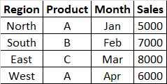
Steps:

1. Create a PivotTable summarizing sales by region and product.
2. Insert a PivotChart linked to the PivotTable.
3. Add slicers for Region and Product.
4. Format the dashboard with a clean layout and clear labels.

Result: A dynamic dashboard where users can filter sales data by region and product in real time.

Interactive Excel charts transform static data presentations into dynamic experiences. By incorporating tools like slicers, dropdown menus, and macros, you can create engaging visuals that empower users to explore data their way.

Write Us- Support@virvijay.com.